Algorithm 1&2: Build the prefix array and divergence array
Introduction
At its core, PBWT relies on sorting haplotypes at each site to reveal local similarities and create connections between related haplotypes. This document describes the first two fundamental algorithms:
- Algorithm 1: The conceptual foundation that builds the prefix array by sorting haplotypes based on their reverse prefixes.
- Algorithm 2: The primary practical implementation which constructs both the prefix array and the divergence array in a single pass.
Description
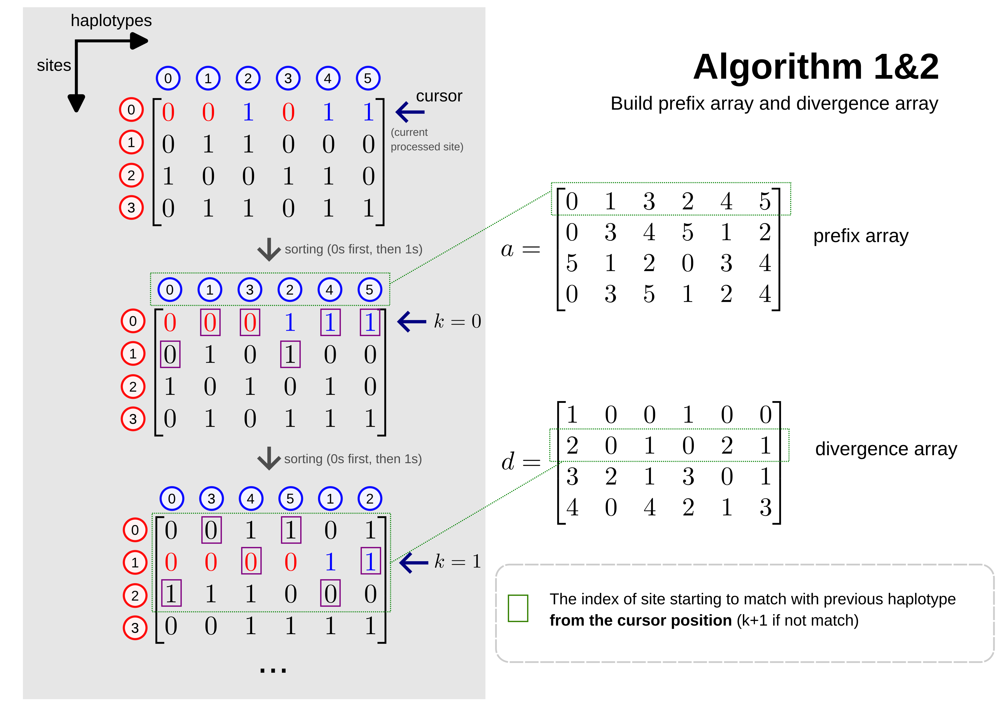
The figure above illustrates the step-by-step process of Algorithms 1 and 2 to construct the prefix array (\(a\)) and the divergence array (\(d\)) from a set of haplotypes.
Haplotype matrix and sorting
Haplotypes are represented as columns, and sites as rows. At each site \(k\) (indicated by the cursor), we sort the haplotypes based on their genotype values (0 or 1). As shown by the grey arrows, this is a stable sort: haplotypes with a 0 at site \(k\) are placed before those with a 1, while their original order is still recognized.
- The top matrix: Shows the initial state at site \(k=0\).
- The middle matrix: Shows the state after sorting at site \(k=0\).
- The bottom matrix: Shows the state after sorting at site \(k=1\).
Prefix array (\(a\))
The matrix \(a\) on the right stores these permutations. Each row \(k\) contains the indices of haplotypes in their sorted order at site \(k\). For example, the haplotypes (columns) are reordered to \([0, 1, 3, 2, 4, 5]\), forming the first row of the prefix array \(a\); and the sort on site 1 reorders the columns to \([0, 3, 4, 5, 1, 2]\), forming the second row of \(a\).
Divergence array (\(d\))
The divergence array \(d\) tracks the length of the matching prefix between adjacent haplotypes in the sorted order. Specifically, \(d_k[i]\) stores the smallest index \(j\) such that haplotype \(a_k[i]\) matches \(a_k[i-1]\) from site \(j\) to site \(k\).
- Purpose boxes: Highlight the site \(j\) that determines the value of \(d_k[i]\). If the haplotypes match at the current site \(k\) and previous sites, the box marks the start of that match.
- Mismatch: If there is no match at the current site \(k\), the divergence is \(k+1\), and the box is shown one row below the cursor.
- Sentinels: For the first haplotype in the sorted order, \(d_k[0]\) is set to \(k+1\) as a sentinel value.
For example, at \(k=1\) (the bottom matrix):
- Haplotype
3follows0. They match at both sites 1 and 0, so \(d_1[1] = 0\). - Haplotype
4follows3. They match at site 1 but differ at site 0. Thus, the match starts at site 1, and \(d_1[2] = 1\). - Haplotype
1follows5. They differ at site 1, so the match is non-existent, and \(d_1[4] = k+1 = 2\).
Conclusion
- Algorithm 2 is the standard implementation used in practice, as it efficiently computes both the prefix and divergence arrays simultaneously.
- In Richard Durbin’s original source code, Algorithm 1 serves as a conceptual starting point, while Algorithm 2 powers the core functionality for later operations.
- The divergence array \(d\) effectively identifies “chains” of shared segments between haplotypes.
- The prefix array \(a\) enables tracing back and grouping similar haplotypes with high efficiency.
- Both algorithms run in linear time \(O(MN)\), processing the \(M \times N\) genotype matrix in a single pass, making the PBWT highly scalable for massive genomic datasets.