Feature selection

Introduction¶

Feature selection is the process of identifying genes that exhibit meaningful biological variability across cells. In scRNA-seq analysis, selecting highly variable genes helps reduce technical noise, improve computational efficiency, and enhance downstream analyses Luecken & Theis, 2019Stuart et al., 2019.

Seurat command

Variance stabilizing transformation

Mean variance plot

Dispersion

pbmc <- FindVariableFeatures(
  pbmc, 
  selection.method = "vst", 
  nfeatures = 2000
)

Methods¶

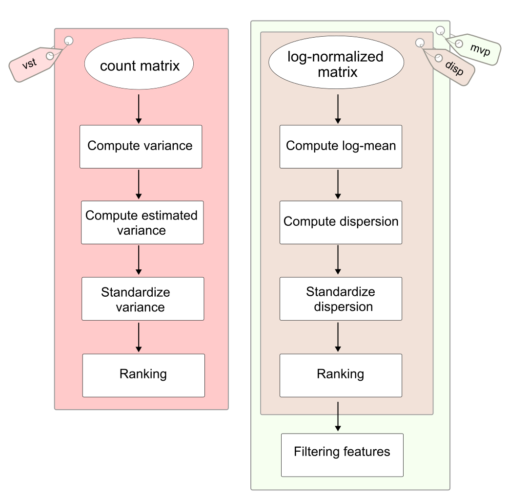
There are three available methods based on two distinct strategies for selecting highly variable features:

Variance stabilizing transformation (vst), which operates directly on the count matrix to estimate and standardize variance for feature ranking.
Mean variance plot (mvp) / Dispersion (disp), which utilize the log-normalized matrix to compute and standardize dispersion values. These dispersion values are subsequently used for gene ranking, while the mvp method additionally incorporates log-mean values to filter qualified features.

Variance stabilizing transformation (`vst`)¶

This method computes standardized variance based on the raw layer input (the count matrix).

\sigma_{i}^2 = \frac{\sum_{j=1}^{N}{(c_{ij} - \mu_{i})^2}}{N-1}

(1)

Firstly, the variance ( $\sigma_{i}^2$ ) corresponding to each gene is computed following the formula (1), where $c_{ij}$ is an element of gene $i$ and cell $j$ in the count matrix; $\mu_{i}$ is the mean of expression count of gene $i$ ; and N is the number of cells.

\hat{\sigma_{i}}^2 = \text{LOESS} \left( \log_{10}(\sigma_i^2) \sim \log_{10}(\mu_i) \right)

(2)

Subsequently, the expected variance ( $\hat{\sigma_{i}}^2$ ) is estimated by the Local Polynomial Regression model (LOESS) Cleveland et al., 2017. The model fits a smooth trend to capture the relationship between gene abundance and variance in log-log space (the formula (2)). Using local parabolic fitting, the expected variance is estimated across the mean expression range to generate a continuous, smooth curve (See brilliant Josh’s explanation).

\begin{cases} \begin{aligned} z_{ij} &= \frac{c_{ij} - \mu_{i}}{\hat{\sigma_{i}}} \\ \bar{\sigma_{i}}^2 &= \frac{\sum_{j=1}^{N}{\left[\min(\sigma_{\text{max}}, z_{ij})\right]^2}}{N-1} \end{aligned} \end{cases}

(3)

Finally, the standardized variance ( $\bar{\sigma_{i}}^2$ ) for gene $i$ is computed by formula (3), which represents the variance of the standardized values ( $z_{ij}$ ) across all cells, capped at a maximum value of $\sigma_{\text{max}} = \sqrt{N}$ , which ensures the balanced distribution of variance, preventing outliers from overwhelmingly escalating the gene’s overall variance.

The genes are then ranked by their standardized variance in descending order to select the top highly variable features (default nfeatures = 2000).

Mean variance plot (`mvp`)¶

The log-normalized matrix is utilized to execute this approach. The workflow begins by computing log-mean ( $\text{log}_{\mu_{i}}$ ) via equation (4) to divide the features into discrete computational bins. Next, the dispersion value for each gene ( $disp_i$ ) is calculated using the system of equations defined in (5). Finally, equation (6) standardizes dispersion based on the mean and standard deviation of its assigned bin. These standardized dispersion values are ultimately used alongside the log-mean values to sort and select the most highly variable features.

\text{log}_{\mu_{i}} = \ln \left( 1 + \frac{1}{N} \sum^{N}_{j=1}{\left(e^{LN_{ij}} - 1\right)} \right)

(4)

The formula (4) reverses the log-normalization step to recover relative count ( $RC_{ij}$ ), calculates the arithmetic mean of these relative counts for each gene, and finally converts the resulting mean back to the log scale using the $\ln(1+x)$ transformation.

The values of log-mean are utilized to divide the genes into distinct bins, where the total number of bins is controlled by the num.bin attribute (which defaults to 20).

\begin{cases} \begin{aligned} \mu_i &= \frac{1}{N} \sum_{j=1}^{N} RC_{ij} \\ \sigma_i^2 &= \frac{1}{N - 1} \sum_{j=1}^{N} \left( RC_{ij} - \mu_i \right)^2 \\ disp_i &= \ln \left( \frac{\sigma_i^2}{\mu_i} \right) \end{aligned} \end{cases}

(5)

Hence, the relationship between the mean and variance of background genes is expected to follow a Poisson distribution, where $\mu_i = \sigma_i^2$ . Consequently, the variance-to-mean ratio (VMR), or Fano factor, for these background features should equal 1. A larger VMR indicates that a gene exhibits greater overdispersion, thereby capturing meaningful biological variability across cells Oberg et al., 2012Wills et al., 2013. The system of equations in (5) models this by calculating dispersion ( $disp_i$ ), defined as the natural logarithm of the VMR of the relative counts.

\overline{disp}_i = \frac{disp_i - \mu_{\text{bin}_k}}{\sigma_{\text{bin}_k}}

(6)

Next, the formula (6) standardizes the dispersion values using the mean and standard deviation of the specific computational bin ( $\text{bin}_k$ ) assigned to each gene based on its log-mean expression. Finally, the genes are sorted in descending order according to these scaled values, and the top features are selected (determined by the nfeatures attribute).

Additionally, these features are filtered based on default threshold ranges: the log-mean expression must fall between 0.1 and 8 (mean.cutoff), and the standardized dispersion must be greater than 1 (dispersion.cutoff).

Dispersion (`disp`)¶

The dispersion mode follows the same procedure as Mean variance plot (mvp), except that features are not filtered according to log-mean and standardized dispersion at the end of the workflow.

Summary¶

Method	Purpose	A-code
Variance stabilizing transformation (default)	Ranks genes by standardized variance	FindVariableFeatures_vst.R
Mean variance plot	Ranks genes exhibiting strong overdispersion relative to a Poisson distribution	FindVariableFeatures_mvp.R
Dispersion	Ranks overdispersed genes using the same approach as the mean variance plot method, without filtering	FindVariableFeatures_disp.R

References¶

Luecken, M. D., & Theis, F. J. (2019). Current Best Practices in Single-cell RNA-seq Analysis: A Tutorial. Molecular Systems Biology, 15(6), MSB188746. 10.15252/msb.20188746
Stuart, T., Butler, A., Hoffman, P., Hafemeister, C., Papalexi, E., Mauck, W. M., Hao, Y., Stoeckius, M., Smibert, P., & Satija, R. (2019). Comprehensive Integration of Single-Cell Data. Cell, 177(7), 1888-1902.e21. 10.1016/j.cell.2019.05.031
Cleveland, W. S., Grosse, E., & Shyu, W. M. (2017). Local regression models. In Statistical models in S (pp. 309–376). Routledge.
Ahlmann-Eltze, C., & Huber, W. (2023). Comparison of Transformations for Single-Cell RNA-seq Data. Nature Methods, 20(5), 665–672. 10.1038/s41592-023-01814-1
Oberg, A. L., Bot, B. M., Grill, D. E., Poland, G. A., & Therneau, T. M. (2012). Technical and Biological Variance Structure in mRNA-Seq Data: Life in the Real World. BMC Genomics, 13(1), 304. 10.1186/1471-2164-13-304
Wills, Q. F., Livak, K. J., Tipping, A. J., Enver, T., Goldson, A. J., Sexton, D. W., & Holmes, C. (2013). Single-Cell Gene Expression Analysis Reveals Genetic Associations Masked in Whole-Tissue Experiments. Nature Biotechnology, 31(8), 748–752. 10.1038/nbt.2642

Introduction¶

Methods¶

Variance stabilizing transformation (vst)¶

Mean variance plot (mvp)¶

Dispersion (disp)¶

Summary¶

Variance stabilizing transformation (`vst`)¶

Mean variance plot (`mvp`)¶

Dispersion (`disp`)¶